3. Define calibration sections
The goal of this notebook is to show how you can define calibration sections. That means that we define certain parts of the fiber to a timeseries of temperature measurements. Here, we assume the temperature timeseries is already part of the xarray.Dataset object.
[1]:
import os
from dtscalibration import read_silixa_files
[2]:
filepath = os.path.join("..", "..", "tests", "data", "double_ended2")
ds = read_silixa_files(directory=filepath, timezone_netcdf="UTC", file_ext="*.xml")
6 files were found, each representing a single timestep
6 recorded vars were found: LAF, ST, AST, REV-ST, REV-AST, TMP
Recorded at 1693 points along the cable
The measurement is double ended
Reading the data from disk
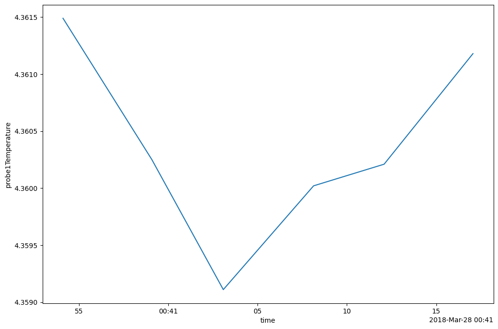
First we have a look at which temperature timeseries are available for calibration. Therefore we access ds.data_vars and we find probe1Temperature and probe2Temperature that refer to the temperature measurement timeseries of the two probes attached to the Ultima.
Alternatively, we can access the ds.dts.get_timeseries_keys() function to list all timeseries that can be used for calibration.
[3]:
# The following line introduces the .dts accessor for xarray datasets
import dtscalibration  # noqa: E401  # noqa: E401

print(ds.dts.get_timeseries_keys())  # list the available timeseeries
ds.probe1Temperature.plot(figsize=(12, 8))
['acquisitionTime', 'referenceTemperature', 'probe1Temperature', 'probe2Temperature', 'referenceProbeVoltage', 'probe1Voltage', 'probe2Voltage', 'userAcquisitionTimeFW', 'userAcquisitionTimeBW']
[3]:
[<matplotlib.lines.Line2D at 0x763e1213dd90>]
A calibration is needed to estimate temperature from Stokes and anti-Stokes measurements. There are three unknowns for a single ended calibration procedure \(\gamma\), \(C\), and \(\alpha\). The parameters \(\gamma\) and \(\alpha\) remain constant over time, while \(C\) may vary.
At least two calibration sections of different temperatures are needed to perform a decent calibration procedure.
This setup has two baths, named ‘cold’ and ‘warm’. Each bath has 2 sections. probe1Temperature is the temperature timeseries of the cold bath and probe2Temperature is the temperature timeseries of the warm bath.
Name section |
Name reference temperature time series |
Number of sections |
Location of sections (m) |
|---|---|---|---|
Cold bath |
probe1Temperature |
2 |
7.5-17.0; 70.0-80.0 |
Warm bath |
probe2Temperature |
2 |
24.0-34.0; 85.0-95.0 |
Sections are defined in a dictionary with its keywords of the names of the reference temperature time series. Its values are lists of slice objects, where each slice object is a section.
Note that slice is part of the standard Python library and no import is required.
[4]:
sections = {
    "probe1Temperature": [slice(7.5, 17.0), slice(70.0, 80.0)],  # cold bath
    "probe2Temperature": [slice(24.0, 34.0), slice(85.0, 95.0)],  # warm bath
}
NetCDF files do not support reading/writing python dictionaries. Internally the sections dictionary is stored in ds._sections as a string encoded with yaml, which can be saved to a netCDF file. Each time the sections dictionary is requested, yaml decodes the string and evaluates it to the Python dictionary.