12. Creating a Dataset from numpy arrays

The goal of this notebook is to demonstrate how to create a xarray.Dataset from scratch. This can be useful if your device is not supported or if you would like to integrate the dtscalibration library in your current routine.

import numpy as np
import os
import matplotlib.pyplot as plt
import xarray as xr

from dtscalibration import read_silixa_files

# The following line introduces the .dts accessor for xarray datasets
import dtscalibration  # noqa: E401  # noqa: E401
from dtscalibration.variance_stokes import variance_stokes_constant

For a xarray.Dataset object, a few things are needed:

• timestamps

• Stokes signal

• anti-Stokes signal

• x (length along fiber)

Let’s grab the data from an existing silixa dataset:

filepath = os.path.join("..", "..", "tests", "data", "single_ended")

ds_silixa = read_silixa_files(directory=filepath, silent=True)

We will get all the numpy arrays from this xarray.Dataset to create a new one from ‘scratch’.

Let’s start with the most basic data:

x = ds_silixa.x.values
time = ds_silixa.time.values
ST = ds_silixa.st.values
AST = ds_silixa.ast.values

Now this data has to be inserted into an xarray Dataset

ds = xr.Dataset()
ds["x"] = ("x", x)
ds["time"] = ("time", time)
ds["st"] = (["x", "time"], ST)
ds["ast"] = (["x", "time"], AST)

print(ds)

<xarray.Dataset> Size: 82kB
Dimensions:  (x: 1461, time: 3)
Coordinates:
  * x        (x) float64 12kB -80.74 -80.62 -80.49 -80.36 ... 104.6 104.7 104.8
  * time     (time) datetime64[ns] 24B 2018-05-04T12:22:17.710000 ... 2018-05...
Data variables:
    st       (x, time) float64 35kB -0.8058 0.4287 -0.513 ... 27.99 27.83 28.81
    ast      (x, time) float64 35kB -0.2459 -0.5932 0.1111 ... 36.2 35.7 35.16

For calibration, a few more paramaters are needed:

• acquisition time (for calculating residuals for WLS calibration)

• reference temperatures

• a double ended flag

We’ll put these into the custom xarray.Dataset:

ds["acquisitiontimeFW"] = ds_silixa["acquisitiontimeFW"].values
ds["userAcquisitionTimeFW"] = ds_silixa["acquisitiontimeFW"].values
ds["temp1"] = ds_silixa["probe1Temperature"]
ds["temp2"] = ds_silixa["probe2Temperature"]

ds.attrs["isDoubleEnded"] = "0"

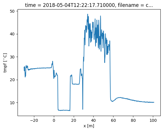
Now we can calibrate the data as usual (ordinary least squares in this example).

ds = ds.sel(x=slice(-30, 101))
sections = {
    "temp1": [slice(20, 25.5)],  # warm bath
    "temp2": [slice(5.5, 15.5)],  # cold bath
}

st_var, resid = variance_stokes_constant(
    ds.dts.st, sections, ds.dts.acquisitiontime_fw, reshape_residuals=True
)
ast_var, _ = variance_stokes_constant(
    ds.dts.ast, sections, ds.dts.acquisitiontime_fw, reshape_residuals=False
)
out = ds.dts.calibrate_single_ended(sections=sections, st_var=st_var, ast_var=ast_var)
out.isel(time=0).tmpf.plot()

[<matplotlib.lines.Line2D at 0x7efbebbf2a00>]