4. Calculate variance of Stokes and anti-Stokes measurements

The goal of this notebook is to estimate the variance of the noise of the Stokes measurement. The measured Stokes and anti-Stokes signals contain noise that is distributed approximately normal. We need to estimate the variance of the noise to: - Perform a weighted calibration - Construct confidence intervals

import os
import warnings

warnings.simplefilter("ignore")  # Hide warnings to avoid clutter in the notebook

from dtscalibration import read_silixa_files

# The following line introduces the .dts accessor for xarray datasets
import dtscalibration  # noqa: E401  # noqa: E401
from dtscalibration.variance_stokes import variance_stokes_constant
from matplotlib import pyplot as plt

filepath = os.path.join("..", "..", "tests", "data", "double_ended2")

ds = read_silixa_files(directory=filepath, timezone_netcdf="UTC", file_ext="*.xml")

6 files were found, each representing a single timestep
6 recorded vars were found: LAF, ST, AST, REV-ST, REV-AST, TMP
Recorded at 1693 points along the cable
The measurement is double ended
Reading the data from disk

And we define the sections as we learned from the previous notebook. Sections are required to calculate the variance in the Stokes.

sections = {
    "probe1Temperature": [slice(7.5, 17.0), slice(70.0, 80.0)],  # cold bath
    "probe2Temperature": [slice(24.0, 34.0), slice(85.0, 95.0)],  # warm bath
}

The variance in the Stokes signal will vary along the length of the fiber. There are multiple ways to approach this, each has its own pros and cons. It is important to consider which model you use for your setup, as this will impact the calibration weights and predicted uncertainty.

• In small setups with small variations in Stokes intensity, variance_stokes_constant can be used. This function determines a single (constant) value for the variance. This method is not recommended for larger setups (e.g., >300 m) due to the signal strength dependency of the variance.

• For larger setups variance_stokes_linear should be used. This function assumes a linear relationship between the Stokes signal strength and variance. Tests on Silixa and Sensornet devices indicate this relationship is linear, and (approximately) goes through the origin; i.e. at 0 Stokes intensity, the signal variance is very close to 0.

• variance_stokes_exponential can be used for small setups with very few time steps. Too many degrees of freedom results in an under estimation of the noise variance. Almost never the case, but use when calibrating e.g. a single time step.

As the setup we are using is only 100 m in length, we can use ds.variance_stokes_constant

I_var, residuals = variance_stokes_constant(
    ds.dts.st, sections, ds.dts.acquisitiontime_fw, reshape_residuals=True
)
print(
    "The variance of the Stokes signal along the reference sections "
    "is approximately {:.2f} on a {:.1f} sec acquisition time".format(
        I_var, ds.userAcquisitionTimeFW.data[0]
    )
)

The variance of the Stokes signal along the reference sections is approximately 8.18 on a 2.0 sec acquisition time

from dtscalibration import plot

fig_handle = plot.plot_residuals_reference_sections(
    residuals,
    sections,
    title="Distribution of the noise in the Stokes signal",
    plot_avg_std=I_var**0.5,
    plot_names=True,
    robust=True,
    units="",
    method="single",
)

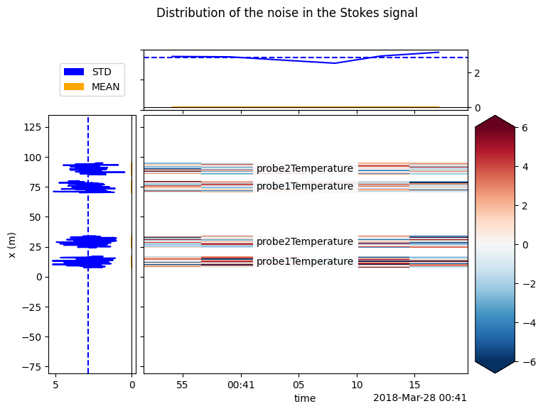
The residuals should be normally distributed and independent from previous time steps and other points along the cable. If you observe patterns in the residuals plot (above), it might be caused by: - The temperature in the calibration bath is not uniform - Attenuation caused by coils/sharp bends in cable - Attenuation caused by a splice

import scipy
import numpy as np

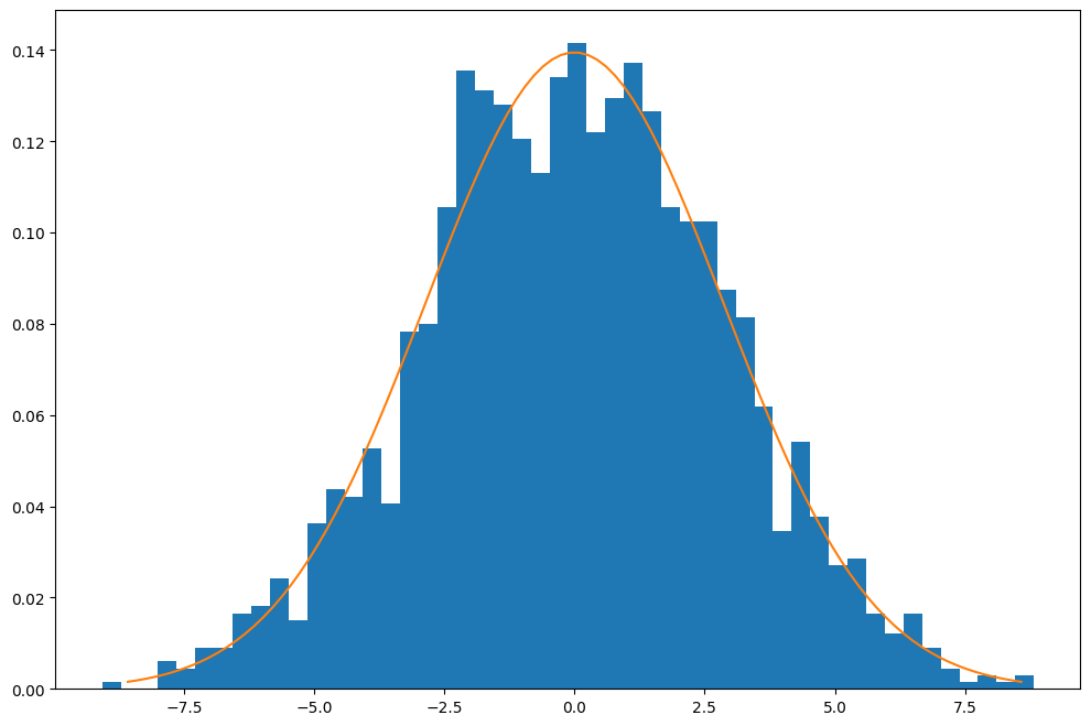
sigma = residuals.std().to_numpy()
mean = residuals.mean().to_numpy()
x = np.linspace(mean - 3 * sigma, mean + 3 * sigma, 100)
approximated_normal_fit = scipy.stats.norm.pdf(x, mean, sigma)
residuals.plot.hist(bins=50, figsize=(12, 8), density=True)
plt.plot(x, approximated_normal_fit)

[<matplotlib.lines.Line2D at 0x7f28a513f310>]

We can follow the same steps to calculate the variance from the noise in the anti-Stokes measurments by setting st_label='ast and redoing the steps.