8. Calibration of double-ended measurements
A double-ended calibration is performed where the unknown parameters are estimated using fiber sections that have a reference temperature. The parameters are estimated with a weighted least squares optimization using Stokes and anti-Stokes measurements from all timesteps. Thus Stokes and anti-Stokes measurements with a large signal to noise ratio (close to the DTS device) contribute more towards estimating the optimal parameter set. This approach requires one extra step, estimating the variance of the noise in the Stokes measurements, but it improves the temperature estimate and allows for the estimation of uncertainty in the temperature. So well worth it!
Double-ended calibration requires a few steps. Please have a look at [1] for more information:
Read the raw data files loaded from your DTS machine
Define the reference fiber sections that have a known temperature
Align measurements of the forward and backward channels
Estimate the variance of the noise in the Stokes and anti-Stokes measurements
Perform the parameter estimation and compute the temperature along the entire fiber
Plot the uncertainty of the estimated temperature
[1]: des Tombe, B., Schilperoort, B., & Bakker, M. (2020). Estimation of Temperature and Associated Uncertainty from Fiber-Optic Raman-Spectrum Distributed Temperature Sensing. Sensors, 20(8), 2235. https://doi.org/10.3390/s20082235
[1]:
import os
import warnings

from dtscalibration import read_silixa_files
from dtscalibration.dts_accessor_utils import (
    suggest_cable_shift_double_ended,
    shift_double_ended,
)

# The following line introduces the .dts accessor for xarray datasets
import dtscalibration  # noqa: E401  # noqa: E401
from dtscalibration.variance_stokes import variance_stokes_constant
import matplotlib.pyplot as plt
import numpy as np

warnings.simplefilter("ignore")  # Hide warnings to avoid clutter in the notebook
Read the raw data files loaded from your DTS machine
Use read_silixa_files for reading files from a Silixa device. The following functions are available for reading files from other devices: read_sensortran_files, read_apsensing_files, and read_sensornet_files. See Notebook 1. If your DTS device was configured such that your forward- and backward measurements are stored in seperate folders have a look at 11Merge_single_measurements_into_double example notebook.
[2]:
filepath = os.path.join("..", "..", "tests", "data", "double_ended2")

ds_notaligned = read_silixa_files(
    directory=filepath, timezone_netcdf="UTC", file_ext="*.xml"
)
6 files were found, each representing a single timestep
6 recorded vars were found: LAF, ST, AST, REV-ST, REV-AST, TMP
Recorded at 1693 points along the cable
The measurement is double ended
Reading the data from disk
Align measurements of the forward and backward channels
In double-ended measurements, it is important that the measurement points of the forward channel are at the same point as those of the backward channel. This requires setting the exact cable length prior to calibration. For double ended measurements it is important to use the correct length so that the forward channel and the backward channel are perfectly aligned. It matters a lot whether your fiber was 99 while in reality it was a 100 meters, as it increases the apparent spatial resolution of your measurements and increases parameter uncertainty and consequently increases the uncertainty of the estimated temperature.
Select the part of the fiber that contains relevant measurements using the sel command. Slice the time dimension to select the measurements of the relevant times.
[3]:
ds_notaligned = ds_notaligned.sel(x=slice(0, 100)) # only calibrate parts of the fiber
The tool suggest_cable_shift_double_ended located in dtscalibration.dts_accessor_utils can be used estimate the required shift to perfectly align the forward and backward channels.
[4]:
suggested_shift = suggest_cable_shift_double_ended(
    ds_notaligned,
    np.arange(-5, 5),  # number of dx to shift
    plot_result=True,
    figsize=(12, 6),
)
print(suggested_shift)
(0, 0)
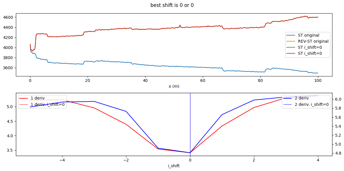
This helper function suggests shift via two different methods. We apply the first suggested shift:
[5]:
ds = shift_double_ended(ds_notaligned, suggested_shift[0])
Define the reference fiber sections that have a known temperature
As explained in Notebook 3. As explained in Notebook 3. DTS devices come with temperature probes to measure the temperature of the water baths. These measurements are stored in the data that was loaded in the previous step and are loaded automatically. In the case you would like to use an external temperature sensor, have a look at notebook 09Import_timeseries to append those measurements to the ds before continuing with the calibration.
[6]:
sections = {
    "probe1Temperature": [slice(7.5, 17.0), slice(70.0, 80.0)],  # cold bath
    "probe2Temperature": [slice(24.0, 34.0), slice(85.0, 95.0)],  # warm bath
}
Estimate the variance of the noise in the Stokes and anti-Stokes measurements
First calculate the variance in the measured Stokes and anti-Stokes signals, in the forward and backward direction. See Notebook 4 for more information.
The Stokes and anti-Stokes signals should follow a smooth decaying exponential. This function fits a decaying exponential to each reference section for each time step. The variance of the residuals between the measured Stokes and anti-Stokes signals and the fitted signals is used as an estimate of the variance in measured signals. This algorithm assumes that the temperature is the same for the entire section but may vary over time and differ per section.
Note that the acquisition time of the backward channel is passed to the variance_stokes function for the later two funciton calls.
[7]:
st_var, resid = variance_stokes_constant(
    ds.dts.st, sections, ds.dts.acquisitiontime_fw, reshape_residuals=True
)
ast_var, _ = variance_stokes_constant(
    ds.dts.ast, sections, ds.dts.acquisitiontime_fw, reshape_residuals=False
)
rst_var, _ = variance_stokes_constant(
    ds.dts.rst, sections, ds.dts.acquisitiontime_bw, reshape_residuals=False
)
rast_var, _ = variance_stokes_constant(
    ds.dts.rast, sections, ds.dts.acquisitiontime_bw, reshape_residuals=False
)
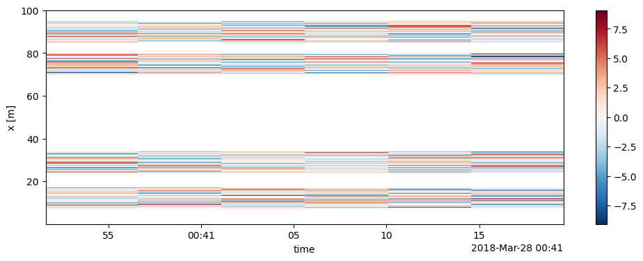
The following plot can be used to check if there are no spatial or temporal correlated residuals. If you see horizontal or vertical lines that means that you overestimate the st_var. Common reasons are that the temperature of that section is not uniform, e.g. that the reference sections were defined falsely (horizontal lines) or that the temperature of the water baths were not uniform (horizontal lines).
[8]:
resid.plot(figsize=(12, 4))
[8]:
<matplotlib.collections.QuadMesh at 0x712669749df0>
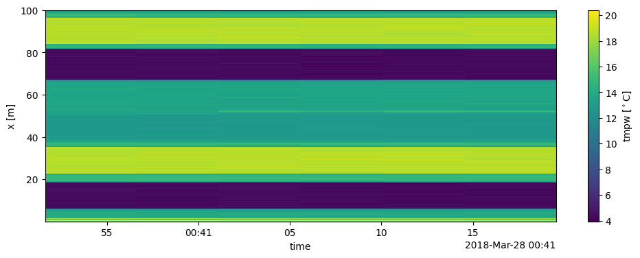
Perform calibration and compute the temperature
We calibrate the measurements with a single method call. Three temperatures are estimated for double-ended setups. The temperature using the Stokes and anti-Stokes meassurements of the forward channel, tmpf. The temperature of the backward channel, tmpb. And the weigthed average of the two, tmpw. The latter is the best estimate of the temperature along the fiber with the smallest uncertainty.
[9]:
out = ds.dts.calibrate_double_ended(
    sections=sections,
    st_var=st_var,
    ast_var=ast_var,
    rst_var=rst_var,
    rast_var=rast_var,
)
[10]:
out.tmpw.plot(figsize=(12, 4))
[10]:
<matplotlib.collections.QuadMesh at 0x71266179eb70>
Uncertainty of the calibrated temperature
The uncertainty of the calibrated temperature can be computed in two manners:
The variance of the calibrated temperature can be approximated using linear error propagation
Very fast computation
Only the variance is estimated
Sufficiently accurate approximation for most cases
The uncertainty distribution of the calibrated temperature can be approximated using Monte Carlo
Slow computation
Computes variances and confidence intervals
Correctly propagates all uncertainties from the calibration
Requires sufficiently large number of samples to be drawn to be correct, hence the slow computation.
Only use this method: 1) To check the first method. 2) Specific interest in confidence intervals.
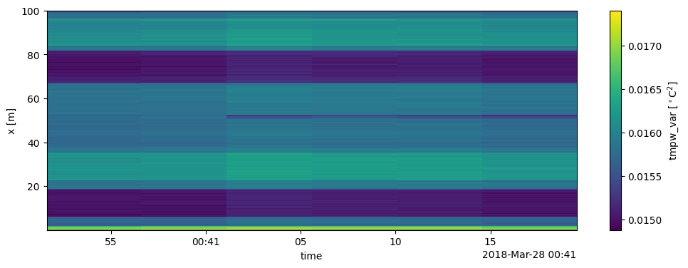
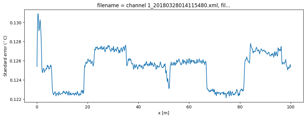
1. The variance approximated using linear error propagation
This first method works pretty good and is always computed when calling the ds.calibration_double_ended() function. First we plot variances for all times. Secondly, we plot the standard deviation (standard error) for the first timestep.
[11]:
out.tmpw_var.plot(figsize=(12, 4))
ds1 = out.isel(time=-1)  # take only the first timestep
(ds1.tmpw_var**0.5).plot(figsize=(12, 4))
plt.gca().set_ylabel("Standard error ($^\circ$C)");
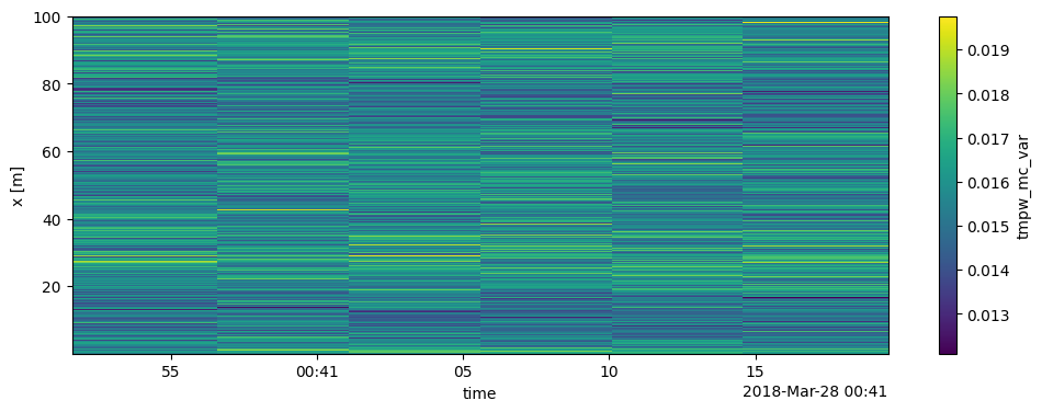
2. Uncertainty approximation using Monte Carlo
If mc_sample_size keyword argument is passed to the ds.calibration_double_ended() function, the uncertainty distribution of the estimated temperature is computed using a Monte Carlo approach. The variance of that distribution is accessed via tmpw_mc_var.
The uncertainty comes from the noise in the (anti-) Stokes measurements and from the parameter estimation. Both sources are propagated via Monte Carlo sampling to an uncertainty distribution of the estimated temperature. As weigths are correctly passed to the least squares procedure via the st_var arguments, the covariance matrix can be used as an estimator for the uncertainty in the parameters. This matrix holds the covariances between all the parameters. A large parameter set is generated
from this matrix as part of the Monte Carlo routine, assuming the parameter space is normally distributed with their mean at the best estimate of the least squares procedure.
The large parameter set is used to calculate a large set of temperatures. By using percentiles or quantile the 95% confidence interval of the calibrated temperature between 2.5% and 97.5% are calculated. The confidence intervals differ per time step. If you would like to calculate confidence intervals temporal averages or averages of fiber sections see notebook 16.
[12]:
out2 = ds.dts.monte_carlo_double_ended(
    result=out,
    st_var=st_var,
    ast_var=ast_var,
    rst_var=rst_var,
    rast_var=rast_var,
    conf_ints=[2.5, 97.5],
    mc_sample_size=500,
)  # < increase sample size for better approximation

out2.tmpw_mc_var.plot(figsize=(12, 4))
[12]:
<matplotlib.collections.QuadMesh at 0x7126616eac60>
[13]:
out.isel(time=-1).tmpw.plot(linewidth=0.7, figsize=(12, 4))
out2.isel(time=-1).tmpw_mc.isel(CI=0).plot(linewidth=0.7, label="CI: 2.5%")
out2.isel(time=-1).tmpw_mc.isel(CI=1).plot(linewidth=0.7, label="CI: 97.5%")
plt.legend(fontsize="small")
[13]:
<matplotlib.legend.Legend at 0x712661552450>
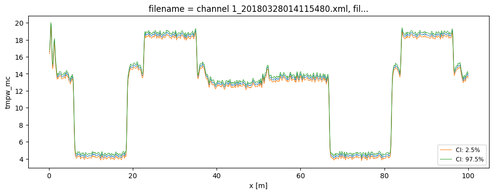
The DataArrays tmpf_mc and tmpb_mc and the dimension CI are added. MC stands for monte carlo and the CI dimension holds the confidence interval ‘coordinates’.
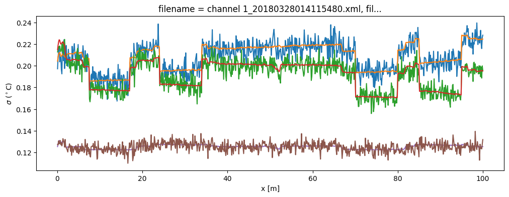
[14]:
(out2.isel(time=-1).tmpf_mc_var ** 0.5).plot(figsize=(12, 4))
(out.isel(time=-1).tmpf_var ** 0.5).plot()
(out2.isel(time=-1).tmpb_mc_var ** 0.5).plot()
(out.isel(time=-1).tmpb_var ** 0.5).plot()
(out.isel(time=-1).tmpw_var ** 0.5).plot()
(out2.isel(time=-1).tmpw_mc_var ** 0.5).plot()
plt.ylabel("$\sigma$ ($^\circ$C)")
[14]:
Text(0, 0.5, '$\\sigma$ ($^\\circ$C)')
[ ]: